


After collecting and annotating the training data, it’s time for model iterations. But what is model training in machine learning? The objective at this stage is to train a model to achieve the best possible performance learning from our annotated dataset. The ultimate goal is a model reaching human-level performance. Such a model can be applied to visual recognition tasks such as self-driving cars.
Model iteration trains models with the annotated dataset and then evaluates the model’s performance. If a model performs great, we can deploy it into production. If the performance is poor, we analyze the root causes to find ways to improve it.
Best Practices for ML Model Training & How-To Guide
Training neural network models is a time consuming process with many decisions:
- What image transformations should I use for data augmentation?
- Which model architecture to use?
- What metrics do I need to evaluate my model?
- Should I use ImageNet pretrained weights on my oil leakage images?
- What hyperparameters do I tune?
Based on our past experience at LandingAI we have developed best practices for model training and evaluation. In this article we share a few high priority tasks during the model training process. We openly share our guiding principles to help machine learning engineers (MLEs) through model training and evaluation.
Review the Image Image Dataset with Examples
Before model training, review the dataset to build a qualitative understanding of the images. After reviewing 100 or more images, major patterns and variance will gradually surface. In particular, look to find answers to the following questions. This will guide selection of image transformations for data augmentation and tuning model configurations.
- Where are the target defects in the image often located?
- If images are to be cropped to be smaller, which region should be retained?
- What is the pixel size of the smallest defects?
- Does the direction or the location of the defect matter in the final prediction?
- How does direction or location of defects affect image selection for data augmentation and postprocessing transformations?
- Is global context needed to determine defects or local features within a 64 x64 pixel window?
- Are the defect class labels easily distinguishable from each other and free of ambiguities?
- Is a class label used less than half of the time?
In our previous article, Data Labeling of Images for Supervised Learning, we recommended MLEs participate in the defect labeling process. When this best practice is followed, MLEs will more easily answer these questions.
MLEs not familiar with the training and dev datasets should scan through the images. Looking closely at the image samples builds understanding of the data. This helps them during model training and error analysis. During model iteration, MLEs should pay attention to how their mind makes predictions and the relevant information used to recognize them. When reviewing model mispredictions, being familiar with the images informs them where errors might be coming.
Train the Model On A Small Set of Data
When starting on a new dataset or a new training pipeline, perform a quick overfitting job. Overfitting trains the model with just a few samples, then evaluates it with those same samples. This is a very easy test and the model is expected to perform perfectly. This quick sanity check ensures the training pipeline is working as expected.
Randomly select a small set of data with five images and run both model training and evaluation on this dataset. Both the training and dev loss curves should converge to zero. We’ll explain the loss curves in a later section of this article.
From our past experience we have found if there’s any mistakes in the training process, the model won’t be able to overfit just five images. Therefore, it is a good sanity check on potential errors in the training process.
After training is complete, run the evaluation and look at the visualized model predictions to see if they match perfectly with the groundtruth labels. If not, it indicates there are some issues on the datasets or the training pipelines. Some possible issues include:
- The cropping coordinates or resize dimensions used in the training job is not consistent with the transforms used in the evaluation job.
- The images or labels are not loaded properly.
- The learning rate is set too high.
Remove all random transformations from the data augmentation when trying to overfit on the data. Keep only transformations needed for inference, such as cropping and resizing.
Selecting Transformations for Data Augmentation
No matter how much data is available, more is always needed to better train machine learning models. Data augmentation is a method to increase the dataset by using existing images then altering them with transformations such as rotating, flipping, cropping, scaling, or adding Gaussian noise. Therefore, data augmentation techniques are highly recommended to increase the variance of training data.
Apply transformations to images in the existing training set. After transformation MLEs must review the resulting images. Here are some considerations that can cause problems.
- The target objects in the images become invisible after resizing.
- Images may become so bright it is impossible to see any objects. This could be due to unreasonably large parameters set as the random brightness transformation.
- For horizontal images at a 3:1 aspect ratio, rotating them randomly by 90 degrees will drop a significant amount of detail. This may introduce unnecessary difficulties for models to fit.
- Applying random blurriness may hinder a model’s capability to detect those defects accurately if the objects are only a few pixels,
Model Hyperparameters
A hyperparameter is a configuration option external to the model. These are values that cannot be determined from the data. Hyperparameters are used to control the speed and quality of the learning process.
Choose backbones and pre-trained weights
A backbone refers to an interchangeable component in the neural network architecture used for feature extraction. Backbones and pre-trained weights are part of the model. Nowadays, changing backbones and weights can be as easy as modifying one parameter in the code. This is a common technique used in object detection and semantic segmentation models. Some popular backbones include ResNet 18, ResNet 34, and VGG 19.
The non-numerical part of the name represents the network architecture (e.g. ResNet, VGG, ResNext). The number indicates the number of layers in the network. The larger the number, the more trainable parameters inside the backbone and the larger the model capacity. However, larger backbones require more training data and the inference latency increases.
The amount of data available in automated visual inspection projects is usually small, around 100 per class. In practice, we typically select a backbone from ResNet 18, ResNet 34, and ResNet 50. We recommend starting from a large network backbone to be sure we can fit with the training data sufficiently. If a severe overfitting issue is found in training, or model latency is a strict requirement, use a smaller backbone.
Backbones for Detecting Defects in Manufacturing
There has not been a thorough review of different model architecture performance in manufacturing data. We do have some research to reference. The transfer performance of 16 popular convolutional architectures on a chest X-ray was tested. These findings were published in Computer Vision and Pattern Recognition, Jan 2021.
The CheXtransfer: Performance and Parameter Efficiency of ImageNet Models for Chest X-Ray Interpretation paper reports newer architectures such as EfficientNet and MobileNet generally underperform older architectures like ResNet. Therefore, we suggest using the ResNet architecture by default.
We highly recommend initializing the model with weightings from COCO or ImageNet datasets. This gives a far better starting point, for much quicker and accurate training. Most of the COCO and ImageNet datasets are animals, furniture, and other common objects in real life. Obviously these are distinctly not defect images in manufacturing. Yet, from experience we found they offer better model performance at training.
This recommendation is validated by the CheXtransfer paper. Researchers found that ImageNet leads to a statistically significant boost in model performance on the medical image dataset.
Effective Image Size for Model Training
To effectively capture small defects, manufacturing images are usually collected with high-resolution industrial cameras. These images are very large files. We have seen many projects where they are over 6.75MB, and larger than 1500×1500 pixels. Such large images slow training and inference. To reduce latency we usually downsize the image in a few ways:
- If interest is only in a specific area, crop the image to the region of interest. Then feed the cropped image into the model.
- Downsize the original image to a reasonable scale. During the initial step of scanning the data set, the smallest defects were found. After downsizing the smallest defects must clearly be visible, occupying at least 5×5 pixels after downsizing.
- If the image is to be passed at its original resolution, crop the image into 16 patches or four rows and four columns. Then batch them to feed into the model. This approach will break the global context in the image. It only works when some local features are needed to predict defects
Hyperparameter Tuning
There are several hyperparameters that can be tuned based on the input data distribution. At LandingAI, we commonly tuned the following hyperparameters based on the data distribution in the training set.
- Class weights tuning in object detection – Weight of each class can be tuned based on its number of samples in the training data relative to other classes.
- Anchor parameters tuning in object detection – Sizes and ratios of anchor boxes can be tuned based on the dimensions of objects in the training set.
- Number of epochs (the number of passes the model has completed for the entire training dataset) – Apply an early stopping technique to the training job when the validation loss converges. Users don’t need to tune the number of epochs for their training jobs.
From our past experience, we have found that a better performance can be achieved with basic hyperparameter tuning on a clean dataset than a time-consuming, expensive parameter searching on a terribly labeled, noisy dataset. Compared with model training, we believe the MLEs time is better spent collecting high quality labels and integrating AI systems. Therefore, we recommend MLEs to invest most of their time on data iterations instead of model iterations.
Evaluation of the Machine Learning Model
Use the Loss Curves to drive decisions
The loss curve is a technique guiding how to tune the training configurations. It plots a model’s loss on a predefined dataset over training time (or the number of epochs). In each of the training jobs, we see one loss curve for the training set (training loss curve) and another for the dev set (dev loss curve), as shown in the figure below:
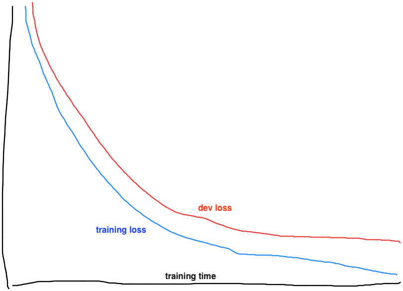
Figure 1: Example training and dev loss curves
Ideally the training loss will converge to a zero loss level. The dev loss curve will closely follow a little above the training loss. This indicates the model has successfully learned the major patterns from the training set. As the training loss approaches zero, the learning is generalized to the dev set. Thus the dev loss is also low. The exact desired loss level will vary based on the loss function used and the variance among datasets.
Loss Curves When Underfitting and Overfitting
If both the training loss curve and the dev loss curve plateau at a high level, consider the model is underfitting. If the training loss curve approaches the zero line while the dev loss curve converges at a high level or goes up, consider the model is overfitting.
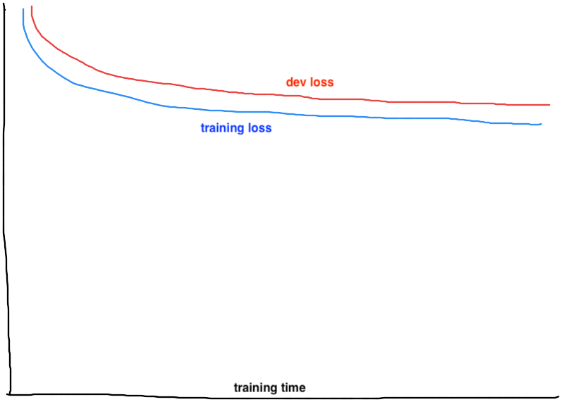
Figure 2: Example loss curve of underfitting |
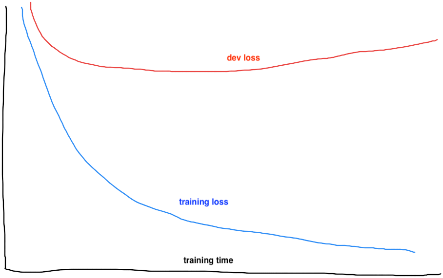
Figure 3: Example loss curve of overfitting |
To address underfitting, try the following techniques.
- Increase the model size (represented by the number of trainable parameters). For example, use a larger model backbone.
- Reduce data augmentation. Review the transformations in the data augmentation to see if they are reasonable. Try removing some of the data augmentation. For example, does randomly rotating images 90 degrees make sense? Was a strong random brightness set that made the image too bright or dark? Did cropping remove some global context necessary for detection?
- Reduce or eliminate regularization. For example, reduce the dropout rate in the model.
- Increase the image size. Maybe the resized image is too small and the target objects are barely detectable. Adjust to a larger image size, yet no larger than the original size.
To address overfitting, try the following techniques.
- Add more training data. The simplest and by far the most effective way to address overfitting.
- Add data augmentation. Review the data augmentation for an increase in the intensity of the existing transformations or add more.
- Decrease the model size. Switch to a smaller model backbone. However, this could hurt model performance and use it with caution. Adding data augmentation and regularization will be better approaches.
Selecting Evaluation Metrics
Common visual recognition tasks may have precision (percentage of positive detections that are relevant) and recall (percentage of relevant positives that are detected), or similar custom metrics, to evaluate models. However, having more than one evaluation metric makes it difficult to compare algorithms.
In the table below, which classifier performance is superior?
| Classifier | Precision | Recall |
| A | 95% | 90% |
| B | 98% | 85% |
During development, try several model hyperparameters and data augmentations. Compare models from different training runs often. A single evaluation metric allows sorting all models on this one dimension.
The table below lists metrics commonly used in computer vision models.
| Use Case | Label Format | Metric |
| Object Detection | Bounding boxes |
|
| Semantic Segmentation | Segmentation map |
|
| Classification | Class |
|
Conclusion
This article describes our best practices and techniques in model training and evaluation. Use this guide to kickstart your first few training jobs. Once you finish evaluation and find your best model, see if it meets your performance targets.
If there are some mispredicted samples, do error analysis to understand the underlying causes and look for ways to improve. Refer to the next article in this series, Boosting Model Performance Through Error Analysis for more information.

